
Synthetic Control in Python: Policy Evaluation Step by Step
Learn synthetic control in Python with a step-by-step policy evaluation of California Proposition 99, including donor weights, placebos, and sensitivity.
Synthetic Control in Python: Policy Evaluation Step by Step
On this page
- What Is the Synthetic Control Method?
- When Should You Use Synthetic Control for Policy Evaluation?
- Synthetic Control vs Difference in Differences
- The Core Math Behind Synthetic Control
- Python Setup and Packages
- Build or Load a Policy Evaluation Dataset
- Inspect the Data Before Fitting the Model
- Choose the Treated Unit and Donor Pool
- Fit the Synthetic Control in Python
- Check Pre Treatment Fit
- Interpret Donor Weights and Predictor Balance
- Estimate the Policy Effect
- Run Placebo Tests Across Units
- Use Time Based or Conformal Inference
- Add Robustness and Sensitivity Checks
- Go Beyond Classic Synthetic Control
- Compare Synthetic Control Variants
- Common Mistakes in Synthetic Control Analysis
- How to Choose the Right Synthetic Control Approach
- Complete Python Workflow
- Results Summary
- Practitioner Takeaways
- Animated View: How the Synthetic Path Is Built
- Frequently Asked Questions
- Conclusion
- References and Further Reading
A policy can change one state, city, hospital, school district, or company before anyone has a clean experiment in place. When that happens, the hardest question is simple: what would have happened without the policy? Synthetic control gives you a practical way to build that missing comparison from several untreated units.
This tutorial shows synthetic control in Python from design to inference. The worked example uses a simulated US state panel and a clean energy policy that starts in 2018. Colorado is the treated state. The values are simulated for teaching. They are not official state statistics, and they should not be used to make a claim about any real Colorado policy.
In the simulated data, the headline model has a pre-treatment RMSE of 0.40 index points. The average post-treatment gap is 9.64 points. Colorado also has the largest post-to-pre RMSPE ratio in the placebo set, which gives a rank-based permutation value of 0.045. Because this is simulated data with a known effect, these numbers are a code check, not real-world evidence.
Core idea
The strongest synthetic control analysis starts with research design, not software. A good plot after treatment cannot rescue a poor donor pool, a weak pre-treatment fit, spillovers, or a policy date chosen after looking at the outcome.
What Is the Synthetic Control Method?
Synthetic control is a causal inference method for settings with one treated unit, or a small number of treated units, and no single untreated unit that works as a convincing comparison. Instead of picking one control state, the method builds a weighted blend of untreated states. That weighted blend is the synthetic control.
The weights are chosen using information from before the policy starts. The goal is to make the synthetic unit look like the treated unit during that pre-treatment period. If the match is close, the synthetic path can serve as an estimate of the outcome that might have occurred without the policy. After treatment, the gap between the actual and synthetic paths is the estimated policy effect.
This idea comes from the synthetic control research developed by Abadie and coauthors. One reason the method is useful in policy work is that the comparison is visible. Readers can inspect the donor weights, the pre-treatment fit, and the post-treatment gap instead of treating the model as a black box.
When Should You Use Synthetic Control for Policy Evaluation?
Synthetic control works best when the design has a clear treated unit and a clear intervention date. It also needs untreated units that were exposed to similar broad forces but were not exposed to the policy being studied. A long pre-treatment history is helpful because it gives the method more information about the treated unit before the intervention.
- Use it when one state or a small group receives a policy while a credible donor pool remains untreated.
- Use it when no single comparison state tracks the treated state well, but a weighted blend can.
- Use it when you have enough pre-treatment periods to judge whether the synthetic path really fits.
- Avoid it when donors are affected by spillovers from the policy, when treatment timing is unclear, or when the outcome definition changes around the policy date.
- Be cautious when the treated unit sits far outside the range of the donor pool. Classic synthetic control uses nonnegative weights that sum to one, so it is built for interpolation rather than extreme extrapolation.
Abadie 2021 stresses that synthetic control should be treated as a research design. The question is not only whether an optimizer can return weights. The question is whether the donor pool and pre-treatment data can support a credible counterfactual.
Synthetic Control vs Difference in Differences
Difference-in-differences and synthetic control solve related problems, but they build the comparison in different ways. A basic difference-in-differences design compares the change in the treated group with the change in a control group. Its key identifying idea is that the groups would have followed parallel trends without treatment.
Synthetic control puts more effort into matching the pre-treatment path. The donor states do not have to receive equal weight. Some may get large weights, while others get zero. This can help when the simple donor average has a different level or trend from the treated unit.
Neither method is automatically better. If a strong parallel trends argument exists and there are many treated and untreated units, difference-in-differences may be simpler and better supported for inference. If one state is treated and a weighted donor blend tracks it very closely before treatment, synthetic control can be easier to defend. Synthetic difference-in-differences combines ideas from both methods and is discussed later.
The Core Math Behind Synthetic Control
Let state 1 be the treated unit. Let the donor pool contain states 2 through J plus 1. For each year t, the outcome for donor state j is Yjt. The synthetic outcome is a weighted average of donor outcomes:
Equation 1
Synthetic_t = sum over donors of w_j times Y_jt
In classic synthetic control, the donor weights are nonnegative and sum to one. That keeps the synthetic unit inside the range created by the donors. The optimizer chooses weights that make the treated and synthetic units close before treatment. A simple outcome matching objective is:
Equation 2
Choose w to minimize the sum of squared pre-treatment differences between Actual_t and Synthetic_t, subject to w_j >= 0 and the weights summing to 1.
You can also match predictors such as income, industrial mix, or electricity prices. In the original framework, a predictor importance matrix called V controls how strongly each predictor matters. The effect in each post-treatment year is then:
Equation 3
Effect_t = Actual_t - Synthetic_t
A positive gap means the treated outcome is above the estimated no policy path. A negative gap means it is below that path. The sign only becomes a policy story after you define the outcome and the expected direction of the policy effect.
Python Setup and Packages
The main workflow below uses NumPy, pandas, SciPy, Matplotlib, and Plotly. It fits classic simplex weights directly with SciPy. This keeps the core method visible and makes it easier to see what the optimizer is doing. The optional conformal section uses the diff diff package because that library provides tested synthetic control inference helpers.
# Environment used for this tutorial build
# Python 3.13.5

numpy==2.3.5
pandas==2.2.3
scipy==1.17.0
matplotlib==3.10.8
plotly==6.5.2
diff-diff==3.11.1
Package APIs change. Before publishing a notebook months from now, check the package release notes and rerun every cell. As of September 3, 2026, PyPI lists diff diff 3.11.1 as the current release. The classic workflow in this article does not depend on that package for the headline estimate.
Build or Load a Policy Evaluation Dataset
A useful policy panel has one row for each unit and time period. In a US state study, the unit might be a state and the time period might be a year or quarter. The outcome should be measured the same way across units and over time. The treatment indicator should turn on only for the treated state after the policy starts.
Our example uses 22 state labels from 2005 through 2024. Colorado is treated starting in 2018. The outcome is a simulated renewable generation index. Three simulated predictors summarize income, industrial share, and electricity price conditions. The treatment effect is added only after 2018 so we can check whether the method recovers it.
Table 1. Data dictionary for the simulated US state policy panel.
| Column | Meaning | Role |
|---|---|---|
| state | US state label | Unit identifier |
| year | 2005 through 2024 | Time variable |
| renewable_index | Simulated index | Outcome |
| treatment | 0 or 1 | Turns on for Colorado in 2018 |
| income_index | Simulated index | Pre-treatment predictor |
| industrial_share | Simulated percent-style measure | Pre-treatment predictor |
| electricity_price_index | Simulated index | Pre-treatment predictor |
import pandas as pd

panel = pd.read_csv("simulated_us_state_panel.csv")
print(panel.shape)
print(panel.head())
print(panel.groupby("state")["year"].agg(["min", "max", "count"]).head())
Data quality
For a real US policy study, replace this simulated panel with an audited source such as an agency data file, a public administrative series, or a reproducible research dataset. Record the source, download date, unit definitions, and any cleaning rules.
Inspect the Data Before Fitting the Model
Do not jump straight to optimization. First check whether each state has the same time coverage, whether the policy date is coded correctly, and whether missing values appear in the pre-treatment period. Plot the treated outcome and the donor outcomes before making any modeling choice.
required = [
    "state", "year", "renewable_index", "treatment",
    "income_index", "industrial_share", "electricity_price_index"
]

assert panel[required].isna().sum().sum() == 0
assert panel.groupby("state")["year"].nunique().nunique() == 1
assert panel.loc[panel["treatment"].eq(1), "state"].nunique() == 1
assert panel.loc[panel["treatment"].eq(1), "year"].min() == 2018
Outliers also matter. A donor with a sudden break before treatment can receive weight for the wrong reason. A predictor measured after treatment can leak policy information into the fit. Keep predictor definitions fixed before you look at post-treatment outcomes.
Choose the Treated Unit and Donor Pool
Donor selection is a design decision. A donor should be untreated during the study window and should not be strongly affected by spillovers from the treated state. It should also have comparable measurement quality and enough pre-treatment history. In a real project, these rules should be written before the final model is fit.
The table below shows a small screening view from the simulated panel. The correlation column is only a descriptive check. It is not a rule for selecting weights. A low correlation can still be useful when several donors combine well, while a high correlation does not prove causal comparability.
Table 2. Example donor screening view.
| Unit | Eligible | Reason | Pre treatment correlation |
|---|---|---|---|
| Idaho | Yes | No simulated contamination or treatment overlap | 0.982 |
| Indiana | Yes | No simulated contamination or treatment overlap | 0.959 |
| Oregon | Yes | No simulated contamination or treatment overlap | 0.953 |
| Nevada | Yes | No simulated contamination or treatment overlap | 0.940 |
| Connecticut | Yes | No simulated contamination or treatment overlap | 0.939 |
| North Carolina | Yes | No simulated contamination or treatment overlap | 0.939 |
| New Mexico | Yes | No simulated contamination or treatment overlap | 0.791 |
| Missouri | Yes | No simulated contamination or treatment overlap | 0.849 |
In real US state work, also review neighboring policy changes, federal programs with uneven state exposure, migration, cross border sales, and regional shocks. If the treated policy can move outcomes in nearby donor states, the no spillover assumption becomes harder to defend.
Fit the Synthetic Control in Python
We now solve for donor weights. The code stacks the pre-treatment outcome history with the three predictors. Each feature is scaled by its standard deviation so a large numeric scale does not dominate the objective. The optimizer is SLSQP with weights bounded between zero and one and a constraint that all weights sum to one.
import numpy as np
from scipy.optimize import minimize

def fit_simplex_weights(X0, X1):
    combined = np.column_stack([X1, X0])
    scale = combined.std(axis=1, ddof=1)
    scale[scale < 1e-12] = 1.0
    X0s = X0 / scale[:, None]
    X1s = X1 / scale

    def objective(w):
        residual = X1s - X0s @ w
        return residual @ residual

    n_donors = X0.shape[1]
    result = minimize(
        objective,
        np.ones(n_donors) / n_donors,
        method="SLSQP",
        bounds=[(0.0, 1.0)] * n_donors,
        constraints={"type": "eq", "fun": lambda w: w.sum() - 1.0},
        options={"maxiter": 5000, "ftol": 1e-10},
    )
    if not result.success:
        raise RuntimeError(result.message)
    return result.x
The headline fit puts the largest weight on Idaho at 0.394. Iowa, Oregon, and New Mexico also receive meaningful weight. Many other states receive little or no weight. This is normal in classic synthetic control because the simplex solution is often sparse.
Table 3. Ten largest donor weights in the headline model.
| Donor state | Weight |
|---|---|
| Idaho | 0.394 |
| Iowa | 0.129 |
| Oregon | 0.111 |
| New Mexico | 0.106 |
| Wisconsin | 0.080 |
| Indiana | 0.075 |
| Connecticut | 0.062 |
| Arizona | 0.012 |
| Mississippi | 0.012 |
| Virginia | 0.010 |
Check Pre-Treatment Fit
Pre-treatment fit is the first result to inspect. If the synthetic unit does not track the treated state before the policy, the post-treatment gap is difficult to interpret. Root mean squared prediction error, often called RMSPE or RMSE in this context, gives a compact measure of the average pre-treatment gap.
For this simulated panel, the pre-treatment RMSE is 0.40 index points. That is small relative to the post-treatment gaps, which reach more than 16.4 points by the end of the sample. The plot also shows that the two paths stay close before 2018.
A low RMSE is useful, but it does not prove the causal design is valid. A model can fit the past well and still fail if donors are contaminated, if the treated state faces a unique shock after treatment, or if the policy date was chosen after searching many dates.
Interpret Donor Weights and Predictor Balance
Donor weights tell you how the synthetic unit is built, but they should not be treated as a unique scientific recipe. Several weight combinations can produce similar pre-treatment paths. The main target is the counterfactual outcome path, not a claim that one specific state contributed exactly a fixed share of causal similarity.
Predictor balance is still useful. It checks whether the weighted donor mix looks closer to the treated state than the raw donor average does on important pre-treatment features. In this example, the synthetic values sit close to Colorado on the three simulated predictors.
Table 4. Predictor balance for treated, synthetic, and raw donor averages.
| Predictor | Treated | Synthetic | Raw donor mean |
|---|---|---|---|
| Income Index | 106.29 | 106.22 | 105.77 |
| Industrial Share | 21.76 | 21.76 | 19.39 |
| Electricity Price Index | 105.35 | 105.32 | 102.40 |
If a key predictor remains badly imbalanced, ask whether the donor pool can support the design. Adding more tuning does not always solve a basic lack of overlap.
Estimate the Policy Effect
The effect path is the actual outcome minus the synthetic outcome. Before treatment, that gap should be close to zero. After treatment, a persistent gap can be evidence of a policy effect if the research design is credible and competing explanations are weak.
In the simulation, the average post-treatment gap is 9.64 index points. The yearly gap starts near 3.43 points in 2018 and rises to 16.41 points in 2024. That rising pattern is expected because the simulated treatment effect was designed to ramp up over time.
In a real study, report both the path and a summary such as the average post-treatment effect. The path can reveal delayed effects, temporary effects, or a break that starts before the official policy date. A single average can hide those patterns.
Run Placebo Tests Across Units
A classic way to assess how unusual the treated gap is is to use in-space placebo tests. Pretend each donor state was treated in 2018, refit a synthetic control for that state, and compute its post-to-pre RMSPE ratio. If Colorado has a much larger ratio than the placebo states, its post-treatment divergence is unusual relative to the donor pool.
Colorado ranks first among all 22 units in this simulation. Its post-to-pre RMSPE ratio is 26.72. The rank-based permutation value is 0.045. With 22 total units, the smallest possible rank value is 1 divided by 22, which is also 0.045. This shows why donor pool size affects the resolution of placebo inference.
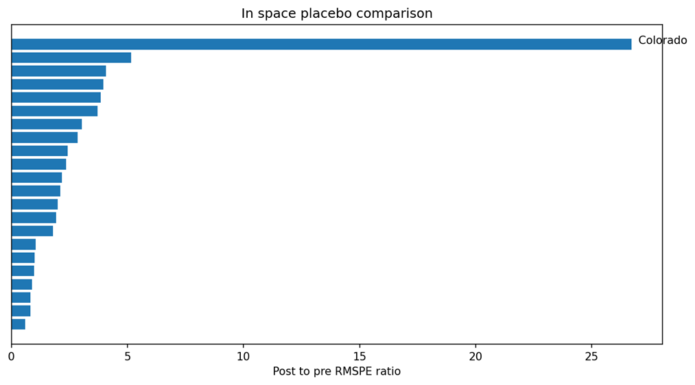 Figure 3. In space placebo ratios. Colorado is the most extreme unit in the simulated panel.
Do not report a placebo value without the pre treatment fit. A placebo state with very poor pre treatment fit can create a large ratio or gap for reasons that have little to do with treatment. Many applied papers show placebo paths only for units with reasonably good pre treatment fit, while also reporting the full rule used for filtering.
Use Time Based or Conformal Inference
Placebo inference compares the treated unit with other units. Conformal inference asks a different question. It compares the post-treatment residual pattern with the treated unit's own time series under a hypothesized effect path. Chernozhukov, Wüthrich, and Zhu developed conformal methods that can handle time dependence through suitable permutation schemes.
The current diff diff documentation exposes three useful result methods for classic synthetic control: conformal_test, conformal_confidence_intervals, and conformal_average_effect. The package fits a time-symmetric proxy model for the conformal procedure, which is not the same fit as the headline predictor weighted synthetic control. That distinction matters because the inference theory requires its own construction.
# Optional conformal workflow with diff-diff 3.11.1
from diff_diff import SyntheticControl

sc = SyntheticControl(v_method="nested", seed=0)
res = sc.fit(
    panel,
    outcome="renewable_index",
    treatment="treatment",
    unit="state",
    time="year",
    predictors=["income_index", "industrial_share", "electricity_price_index"],
)

joint = res.conformal_test(0.0)
pointwise = res.conformal_confidence_intervals(
    alpha=0.10,
    scheme="moving_block",
)
average_ci = res.conformal_average_effect(
    alpha=0.10,
    scheme="moving_block",
)
Inference warning
Do not copy a conformal confidence interval from a different fit and attach it to your manual estimate. Run the inference procedure on the same cleaned panel, record the package version, and explain that conformal and in space placebo inference answer different questions.
Add Robustness and Sensitivity Checks
A credible synthetic control result should not depend on one fragile modeling choice. Useful checks include leaving out high weight donors, changing the pre treatment window, changing predictor sets, and backdating the intervention to a time when no effect should exist. These checks do not prove the design. They show whether the conclusion falls apart under reasonable alternatives.
Table 5. Robustness checks for the simulated policy example.
| Specification | Pre treatment RMSE | Average post treatment effect | Post to pre RMSPE ratio | Conclusion |
|---|---|---|---|---|
| Headline model | 0.40 | 9.64 | 26.72 | Same direction and similar size |
| Start pre period in 2008 | 0.43 | 9.84 | 25.08 | Same direction and similar size |
| Outcome history only | 0.34 | 10.40 | 33.10 | Same direction and similar size |
| Leave out Idaho | 0.49 | 8.65 | 19.21 | Same direction and similar size |
| Leave out Iowa | 0.42 | 10.33 | 27.20 | Same direction and similar size |
| Leave out Oregon | 0.40 | 8.88 | 24.14 | Same direction and similar size |
The effect remains positive and similar across these specifications. Removing Idaho weakens the pre treatment fit, which is expected because Idaho carries the largest headline weight, but the post treatment conclusion remains in the same direction. In real work, a large change after dropping one donor should be discussed, not hidden.
Go Beyond Classic Synthetic Control
Classic synthetic control is only the first step in a larger family of methods. Extensions can help when pre treatment fit is imperfect, when level differences remain, or when you want to combine synthetic weighting with a difference in differences style adjustment.
- Demeaned synthetic control focuses more on changes around unit means. Ferman and Pinto study this idea when pre treatment fit is imperfect.
- Synthetic difference in differences adds unit weights and time weights to a difference in differences style estimator. Arkhangelsky and coauthors developed this method for panel settings.
- Matching and synthetic control, often shortened to MASC, first uses matching to narrow the donor set and then applies synthetic control ideas. The goal is to trade off interpolation and extrapolation risks.
- Augmented synthetic control adds an outcome model correction when the classic weighted blend leaves imbalance. Ben Michael, Feller, and Rothstein show how regression adjustment can reduce bias from imperfect fit.
A more complex estimator is not automatically better. Start with the research design and the fit problem. Then choose an extension that addresses a specific weakness you can name.
Compare Synthetic Control Variants
Table 6. Practical comparison of common synthetic control variants.
| Method | Best use case | Main idea | Inference | Strength | Caution |
|---|---|---|---|---|---|
| Classic synthetic control | One treated unit with strong donor overlap | Nonnegative donor weights that sum to one | In space placebo and related randomization methods | Transparent counterfactual path | Can struggle with imperfect fit |
| Demeaned synthetic control | Level differences remain before treatment | Match deviations around unit means | Method specific inference | Can reduce bias from level mismatch | Still needs a credible donor structure |
| Synthetic difference in differences | Panel data with few treated units | Combines unit and time weighting | Asymptotic, bootstrap, or package supported options | Blends DiD and synthetic weighting | Assumptions differ from classic SC |
| MASC | You want matching before synthetic weighting | Match first, then synthesize | Depends on implementation | Can limit poor comparisons | Results can depend on the matching grid |
| Augmented synthetic control | Classic fit leaves imbalance | Synthetic weights plus regression correction | Method specific inference | Can correct imperfect fit | May use negative effective weights and more modeling |
The comparison table is a starting point, not a scoring system. If classic synthetic control fits the pre treatment path closely and the design is clean, adding a more complex estimator may add little. If classic fit is poor, the right answer may be a different estimator, a different donor pool, or no causal claim at all.
Common Mistakes in Synthetic Control Analysis
- Choosing donors after looking at the post treatment result.
- Using too few pre treatment periods to judge whether the counterfactual fit is stable.
- Treating the largest donor weights as the only states that matter scientifically.
- Ignoring spillovers or other policies that affect donor states.
- Tuning predictors with post treatment information.
- Reporting a large post treatment gap even when pre treatment fit is weak.
- Hiding solver settings, package versions, or failed optimization runs.
- Treating a placebo value as an ordinary regression p value with a large sample approximation.
- Claiming causality because the chart looks convincing without discussing design assumptions.
One more mistake is specification searching. Synthetic control offers many choices about predictors, donor rules, and time windows. Ferman, Pinto, and Possebom show why researchers should be careful about cherry picking specifications. Write important choices down before checking which one produces the largest effect.
How to Choose the Right Synthetic Control Approach
A simple decision order helps. First ask whether the policy design is suitable for a comparative case study. Second ask whether the donor pool can reproduce the treated unit before treatment. Third decide what kind of inference stakeholders need. Fourth check whether the answer is stable to reasonable changes.
- If pre treatment fit is strong and the donor pool is credible, start with classic synthetic control.
- If a level mismatch remains but trends line up, consider a demeaned approach and explain why.
- If you have a panel with few treated units and want a DiD style adjustment, consider synthetic difference in differences.
- If the treated unit is hard to represent with the full donor pool, a matching step may help, but document the matching rule.
- If classic fit is imperfect and an outcome model is defensible, augmented synthetic control may be useful.
- If none of these approaches create a credible pre treatment comparison, report that limitation instead of forcing an estimate.
Complete Python Workflow
The code below is a compact version of the full manual workflow. It assumes the simulated CSV created for this tutorial is in the working directory. For a real project, replace the file and column names, then add your documented donor exclusions before fitting.
import numpy as np
import pandas as pd
from scipy.optimize import minimize
import matplotlib.pyplot as plt

panel = pd.read_csv("simulated_us_state_panel.csv")
treated_state = "Colorado"
policy_year = 2018
predictors = ["income_index", "industrial_share", "electricity_price_index"]

wide = panel.pivot(index="year", columns="state", values="renewable_index")
years = wide.index.to_numpy()
donor_states = [c for c in wide.columns if c != treated_state]
pre = years < policy_year
post = years >= policy_year

X0_outcome = wide.loc[pre, donor_states].to_numpy()
X1_outcome = wide.loc[pre, treated_state].to_numpy()

pred = panel.drop_duplicates("state").set_index("state")[predictors]
X0 = np.vstack([X0_outcome, pred.loc[donor_states].T.to_numpy()])
X1 = np.concatenate([X1_outcome, pred.loc[treated_state].to_numpy()])

combined = np.column_stack([X1, X0])
scale = combined.std(axis=1, ddof=1)
scale[scale < 1e-12] = 1.0
X0s = X0 / scale[:, None]
X1s = X1 / scale

def objective(w):
    residual = X1s - X0s @ w
    return residual @ residual

result = minimize(
    objective,
    np.ones(len(donor_states)) / len(donor_states),
    method="SLSQP",
    bounds=[(0.0, 1.0)] * len(donor_states),
    constraints={"type": "eq", "fun": lambda w: w.sum() - 1.0},
    options={"maxiter": 5000, "ftol": 1e-10},
)
if not result.success:
    raise RuntimeError(result.message)

w = result.x
synthetic = wide[donor_states].to_numpy() @ w
actual = wide[treated_state].to_numpy()
gap = actual - synthetic
pre_rmse = np.sqrt(np.mean(gap[pre] ** 2))
post_rmse = np.sqrt(np.mean(gap[post] ** 2))
average_effect = gap[post].mean()
rmspe_ratio = post_rmse / pre_rmse

weight_table = pd.DataFrame({"state": donor_states, "weight": w})
weight_table = weight_table.sort_values("weight", ascending=False)
print(weight_table.head(10))
print("Pre treatment RMSE:", round(pre_rmse, 3))
print("Average post treatment effect:", round(average_effect, 3))
print("Post to pre RMSPE ratio:", round(rmspe_ratio, 3))

plt.figure(figsize=(9, 5))
plt.plot(years, actual, label="Colorado actual")
plt.plot(years, synthetic, label="Synthetic Colorado")
plt.axvline(policy_year, linestyle=":", label="Policy starts")
plt.legend()
plt.show()

plt.figure(figsize=(9, 5))
plt.plot(years, gap, label="Estimated gap")
plt.axhline(0)
plt.axvline(policy_year, linestyle=":", label="Policy starts")
plt.legend()
plt.show()
When run on the tutorial data, this workflow produces a pre treatment RMSE near 0.396, an average post treatment effect near 9.641, and a post to pre RMSPE ratio near 26.719. Small numeric differences can appear across SciPy versions or solver tolerances, so save your environment and output with the project.
Results Summary
Table 7. Headline results from the simulated policy analysis.
| Diagnostic | Result | Reading |
|---|---|---|
| Pre treatment RMSE | 0.396 | Close pre treatment fit |
| Average post treatment effect | 9.641 index points | Positive simulated effect |
| Post to pre RMSPE ratio | 26.72 | Large rise in error after treatment |
| Placebo rank | 1 of 22 | Most extreme unit |
| Rank based permutation value | 0.045 | Resolution limited by donor count |
| Largest donor weight | Idaho at 0.394 | Sparse donor mix |
| Robustness | Stable direction across listed checks | No single listed check reverses the conclusion |
The plain English reading is straightforward. The synthetic path tracks Colorado closely before the policy. The actual outcome then rises above the synthetic path after 2018. That gap is unusually large when compared with the placebo states, and it stays positive across the listed robustness checks. Because the data are simulated, this is exactly what we hoped to recover.
Practitioner Takeaways
- Design the donor pool before you focus on the estimate.
- Show the pre treatment fit before you discuss the post treatment effect.
- Report the outcome path and the gap path, not only one average number.
- Use predictor balance as a diagnostic, not as proof of identification.
- Run in space placebos and explain the p value resolution created by donor count.
- Use leave one out and time based checks to find fragile specifications.
- Use conformal inference when period level uncertainty is important and the design has enough time information.
- Keep package versions, solver settings, data sources, and exclusions in the published notebook.
Animated View: How the Synthetic Path Is Built
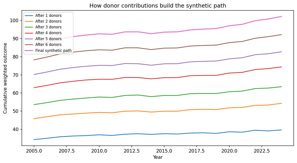
The animated chart in the HTML version adds donor states one at a time in order of their fitted weight. It shows how the weighted donor outcomes accumulate into the final synthetic path. The animation is a teaching aid. It does not mean the optimizer adds states in this order during estimation.
Frequently Asked Questions
How many donor states do I need for synthetic control?
There is no fixed minimum that works for every study. You need enough credible untreated units to build a close pre treatment match. More donors can improve flexibility and give finer placebo inference, but weak or contaminated donors do not become useful just because there are many of them.
How long should the pre treatment period be?
Longer is usually better when the measurement is stable. A long pre treatment period gives you more chances to see whether the synthetic unit tracks the treated unit across changing conditions. The right length depends on the data frequency and the policy setting.
Can synthetic control use negative weights?
Classic synthetic control normally uses nonnegative weights that sum to one. Some extensions and regression based approaches allow negative effective weights. Those methods can reduce imbalance, but they also allow extrapolation and require a different interpretation.
What if my data have missing years?
First find out why the values are missing. Do not fill gaps automatically. Synthetic control relies on comparable histories across units. If missingness is limited, you may use a common balanced window. If it is extensive, the design may not be suitable without a careful missing data plan.
Can I use synthetic control with several treated states?
Yes, but the method and inference need to match that design. You can study treated units separately in some settings, or use extensions built for multiple treated units. Synthetic difference in differences is one option for panel designs with few treated units.
Is synthetic control better than difference in differences?
Not in every case. Synthetic control is attractive when one treated unit can be closely matched by a weighted donor blend. Difference in differences can be better when there are many treated and control units and a strong parallel trends argument. The design should choose the method.
What does a low pre treatment RMSPE tell me?
It tells you the synthetic path tracks the treated outcome closely before treatment. That is necessary for a convincing synthetic control study, but it is not enough by itself. You still need a credible donor pool, no important spillovers, stable measurement, and a clear policy date.
How should I report statistical uncertainty?
For classic synthetic control with one treated unit, use design based tools such as in space placebos, test inversion, and conformal inference when appropriate. Do not invent a standard regression error if the estimator does not provide one.
Conclusion
Synthetic control in Python is most useful when a policy changes one unit and no single untreated unit is a convincing comparison. The method builds a synthetic counterfactual from weighted donors, then compares the treated outcome with that counterfactual after the policy begins.
The workflow is more than an optimizer. Start with a credible donor pool. Check the pre treatment fit. Inspect predictor balance. Plot the effect path. Run placebo inference. Test donor and time window sensitivity. Then decide whether the design supports a causal statement.
In this simulated US state example, the method recovers the known positive policy effect and passes the planned diagnostics. In real policy work, the hardest part is not producing the chart. It is showing that the no policy counterfactual is believable enough for the chart to mean something.
References and Further Reading
- Abadie, Alberto. 2021. Using Synthetic Controls: Feasibility, Data Requirements, and Methodological Aspects. Journal of Economic Literature 59(2), 391 to 425. Source
- Abadie, Alberto, Alexis Diamond, and Jens Hainmueller. 2010. Synthetic Control Methods for Comparative Case Studies: Estimating the Effect of California Tobacco Control Program. Journal of the American Statistical Association. Source
- Arkhangelsky, Dmitry, Susan Athey, David Hirshberg, Guido Imbens, and Stefan Wager. 2021. Synthetic Difference in Differences. American Economic Review 111(12), 4088 to 4118. Source
- Ben Michael, Eli, Avi Feller, and Jesse Rothstein. 2021. The Augmented Synthetic Control Method. Journal of the American Statistical Association 116(536), 1789 to 1803. Source
- Chernozhukov, Victor, Kaspar Wuthrich, and Yinchu Zhu. 2018. Exact and Robust Conformal Inference Methods for Predictive Machine Learning with Dependent Data. Proceedings of Machine Learning Research 75, 732 to 749. Source
- Ferman, Bruno, and Cristine Pinto. 2021. Synthetic Controls with Imperfect Pretreatment Fit. Quantitative Economics 12(4), 1197 to 1221. Source
- Firpo, Sergio, and Vitor Possebom. 2018. Synthetic Control Method: Inference, Sensitivity Analysis and Confidence Sets. Journal of Causal Inference 6(2). Source
- Kellogg, Maxwell, Magne Mogstad, Guillaume Pouliot, and Alexander Torgovitsky. 2021. Combining Matching and Synthetic Control to Trade off Biases from Extrapolation and Interpolation. Journal of the American Statistical Association 116(536), 1804 to 1816. Source
- Carlos Mendez. The Synthetic Control Ladder in Python: A Guided Tour of mlsynth on the Brexit Referendum. Updated August 3, 2026. Source
- diff diff documentation. Synthetic control for a policy evaluation: two routes to inference. Source
- Matheus Facure. Causal Inference for the Brave and True, Chapter 15: Synthetic Control. Source
- Tomas Jancovic. You Did Not Conduct an A B Test. You Can Still Simulate One Retrospectively. TDS Archive, 2024. Source
Downloads
Files attached to this article for your reference.